Final project: a strategy you can check
Build your own adjustable strategy and examine its signals, trades, and results.
The final project brings the parts you have learned into one file: moving averages, inputs, conditions, a custom function, orders, and display. The goal is a program whose every decision you can trace back to data and written rules.
Describe the program without code
The strategy watches two EMAs for crossings. It also uses a third, longer SMA to check whether the closing price is above the average.
A long entry requires the fast EMA to cross above the slow EMA from below and the closing price to be above the trend-filter SMA. The three lengths must follow the order fast < slow < trend. If the supplied lengths do not meet this rule, the program submits no entry order.
The long position receives a market close at a downward EMA crossing. The entry also has a stop and target specified in ticks. The simulation uses a fixed quantity of one unit, 0.1 percent commission, and two ticks of slippage.
These are the task’s rules. We do not infer from them that the program will be profitable on any market. We use the book’s fixed demo data for checking.
The complete program
Create final_strategy.py:
"""
@pyne edge
"""
from pynecore.lib import close, color, input, location, plot, plotshape, script, shape, strategy, ta


def lengths_are_ordered(fast: int, slow: int, trend: int) -> bool:
    return fast < slow and slow < trend


@script.strategy(
    "Filtered Crossing Strategy",
    overlay=True,
    initial_capital=10000,
    default_qty_type=strategy.fixed,
    default_qty_value=1,
    pyramiding=1,
    commission_type=strategy.commission.percent,
    commission_value=0.1,
    slippage=2,
)
def main(
    fast_length: int = input.int(9, title="Fast EMA length", minval=1, maxval=200),
    slow_length: int = input.int(21, title="Slow EMA length", minval=1, maxval=200),
    trend_length: int = input.int(50, title="Trend SMA length", minval=1, maxval=200),
    use_trend_filter: bool = input.bool(True, title="Use trend filter"),
    stop_ticks: int = input.int(100, title="Stop distance (ticks)", minval=1),
    target_ticks: int = input.int(200, title="Target distance (ticks)", minval=1),
):
    fast_average = ta.ema(close, fast_length)
    slow_average = ta.ema(close, slow_length)
    trend_average = ta.sma(close, trend_length)
    crosses_up = ta.crossover(fast_average, slow_average)
    crosses_down = ta.crossunder(fast_average, slow_average)
    valid_lengths = lengths_are_ordered(fast_length, slow_length, trend_length)
    trend_passes = not use_trend_filter or close > trend_average
    entry_signal = valid_lengths and crosses_up and trend_passes
    if entry_signal:
        strategy.entry("Long", strategy.long)
    if crosses_down:
        strategy.close("Long")
    strategy.exit("Bracket", "Long", loss=stop_ticks, profit=target_ticks)
    plot(fast_average, "Fast EMA", color=color.blue, linewidth=2)
    plot(slow_average, "Slow EMA", color=color.orange, linewidth=2)
    plot(trend_average, "Trend SMA", color=color.gray, linewidth=2)
    plotshape(entry_signal, "Entry signal", style=shape.triangleup,
              location=location.belowbar, color=color.green)
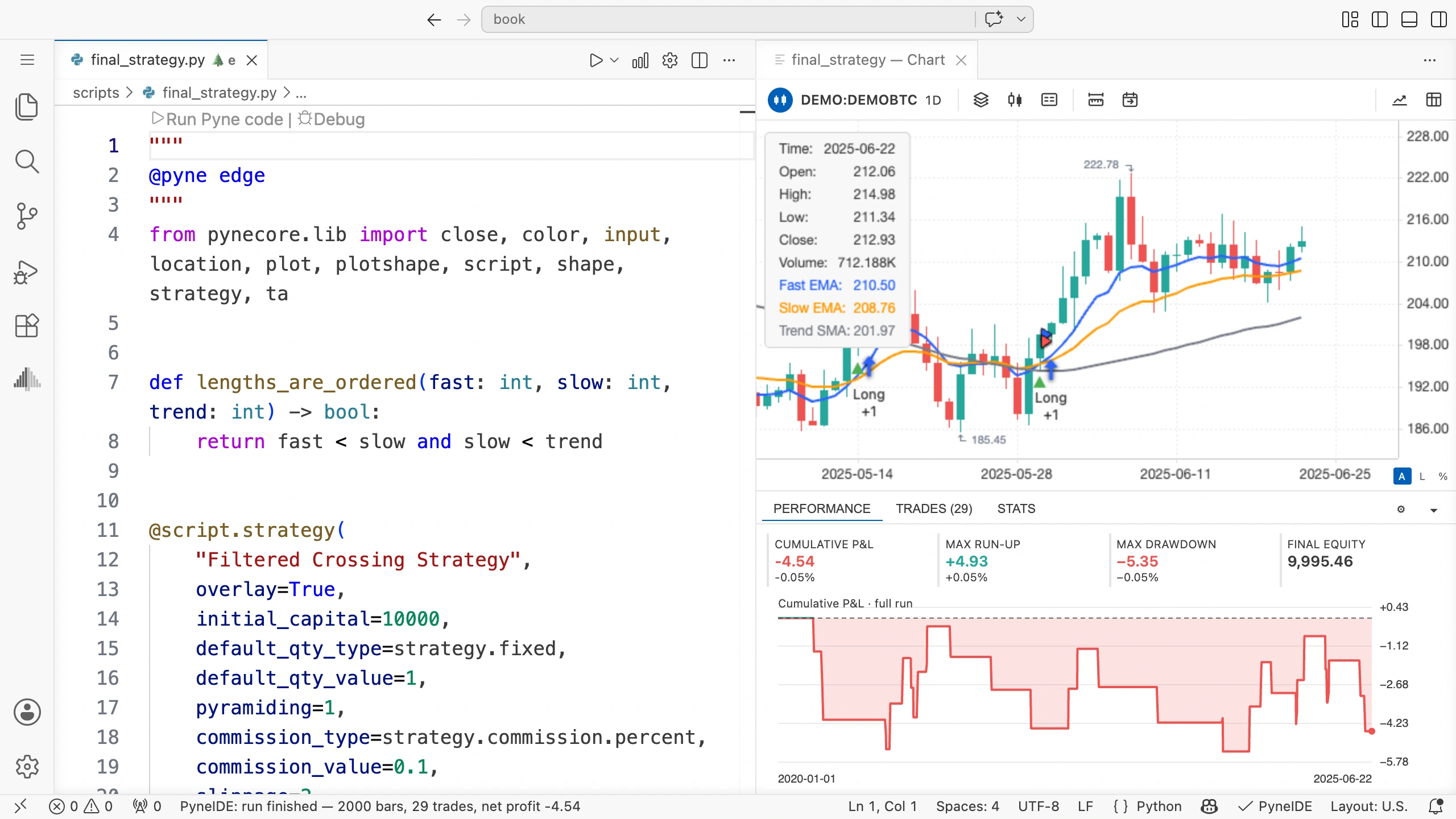
Save it and run it on the demo data. The chart shows three averages and green triangles marking the entry condition. The strategy’s trade markers show actual entries and exits.
What is calculated on every candle?
The three averages and two crossing calculations run before the conditions. We calculate them even if the filter eventually prevents entry. Their calculation state therefore advances across the entire candle sequence.
The custom lengths_are_ordered function examines three numbers and returns a Boolean value. It has no candle state of its own. valid_lengths holds the current result of that check for later expressions.
trend_passes is true if the filter is off or the close is above the SMA. input.bool provides a Boolean input you can toggle. not use_trend_filter is true when the filter is off, so the second condition is not needed then.
When the filter is off, we still calculate and plot the average. The switch changes the entry check, not the line’s display.
An invalid relationship between lengths
The individual input limits say only that each length must be between 1 and 200. You can still enter a fast length of 30 and a slow length of 10. That breaks the order required by the task.
The checking function therefore tests the relationship separately. With the wrong order, the lines still appear, but entry_signal cannot be true. This prevents the program from submitting entries with a length relationship outside the task’s rules.
You can check this directly with valid_lengths in the debugger. The condition stays false throughout the run if the saved inputs are unsuitable.
A signal does not always create a new trade
The green triangle marks the entry condition. The strategy submits the order to the simulator. A fill can have additional requirements: for example, a following candle, sufficient capital, and an allowed quantity.
With pyramiding=1, the simulator may not allow another long entry when a long position is already open. Do not automatically assume the signal count equals the trade count.
At the start of the data, the trend filter’s length-fifty SMA is still missing. With the filter on, we cannot consider the price to be above it yet, so the entry does not meet that condition.
Check the behavior
Start with the defaults and check quantity, costs, and fill behavior in Properties. An override saved earlier can change a setting from the source.
Find a green signal. Using the debugger or chart values, examine both EMAs on that candle and the preceding one. Check the fast/slow crossing, the SMA filter, and the length relationship. All three parts must be true.
Then find the associated entry in Trades. Check which candle it filled on and at what price. For the exit, check whether a crossing, stop, or target explains the close.
Try cases you can predict
To check behavior, make changes whose effects you can predict:
| Change | What should you check? |
|---|---|
| Equal fast and slow lengths | The length check prevents new entry signals |
| Trend filter off | The EMA crossing does not require price above the SMA |
| Larger stop/target distances | The distance change can produce a different exit candle |
| Different quantity | Price signals stay the same; monetary trade size can vary |
Make only one such change per run. For each trial, write down your expectation first and the actual result afterward. If they disagree, find the first different decision in the debugger.
Compare results
When comparing the filter on and off, keep the data, quantity, costs, and lengths the same. Look at the Performance equity curve alongside Trades. A small trade count or a final position still open also affects the summary.
When examining the program on real historical data, record the tuning period and a separate validation period before looking at results. If you change parameters after viewing the validation period, that period also becomes part of the tuning process.
The start of the input data needs enough warmup candles. If you run an extracted period separately, you rebuild the moving averages and position state. The beginning of that separate run can therefore differ from the result for the same period in the middle of a longer dataset.
Try it yourself
Add a Use crossings exit switch to the program. With it on, keep the downward-crossing close; with it off, let only the stop and target close the position. Calculate the downward crossing in both cases.
Solution
In the parameter list of main():
use_crossing_exit: bool = input.bool(True, title="Use crossings exit"),The closing branch:
if use_crossing_exit and crosses_down:
    strategy.close("Long")
Keep crosses_down = ta.crossunder(...) before the conditions. The strategy.exit call remains in both switch positions.
With the crossing-based close off, a position may remain open after a downward EMA crossing. The next entry signal can still appear even though the existing position prevents a new trade from opening.
Create your own version
Copy the program under a new name and describe one new rule you want to add. Specify which data and which candle it uses to decide, how to check it by hand, and which input changes it.
Calculate the new rule as a separate variable first. Plot it or inspect it in the debugger before making it an entry or exit condition. This lets you investigate an error in the calculation before trying to explain the whole strategy’s results.
The source, saved settings, and data together describe your experiment. Keeping them makes the run reproducible and checkable.