Advanced: how do indicators work?
Learn from the source of SMA, EMA, RSI, MACD, ATR, and Bollinger Bands, then create your own indicator variant.
An indicator is easier to adapt when you understand how it produces its value. What goes into the calculation? What does it remember for the next candle? What changes if you use a different average or price source? The source code can answer these questions too.
PyneCore’s ta library is written in Pyne code. The Persistent variables, function calls, and conditions you find there use the behavior you learned in this book. The full source is available, so you can follow a built-in indicator just as you would your own program.
This advanced chapter teaches you how to read source and experiment with it. You do not need to understand the whole library at once. Start with a short function, then follow the calls it depends on.
Open the actual implementation
- Open the
moving_averages.pyfile you created earlier in PyneIDE. - On the
ta.ema(close, 10)line, hold Command on macOS or Ctrl on Windows or Linux and clickema. You can also use Go to Definition in the context menu. - The editor opens the installed PyneCore’s
ta.pyat the definition ofema. - Read the function’s description and then its body. If it calls another function, you can jump to that function’s definition too.
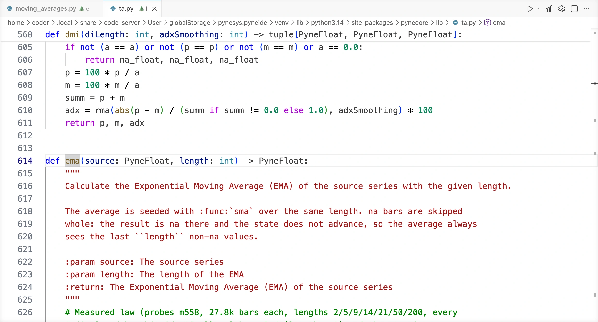
You already tried viewing parameters and jumping to definitions in Help while writing code. The same action takes you to the source for RSI, MACD, and the other library functions. The full ta reference helps you find functions and understand their parameters.
Library code and Edge: at the start of ta.py, you find an @pyne lib marker. The library is not written within Edge’s restricted rules: it also uses general Python tools, internal helpers, and additional type annotations. Its candle-by-candle behavior and state handling will still be familiar. For example, PyneFloat is the library’s numeric type annotation, and na_float means a missing numeric value.
The source excerpts below show the library’s calculations; they are not complete Edge programs. For your own Edge version, express the algorithm you have understood using the allowed tools. Leave the installed ta.py file as it is and experiment in your own files.
SMA: the sum behind the formula
Two lines from the ta.sma calculation:
length = int(length)
return lib_math.sum(source, length) / length
The average is the window’s sum divided by its element count. After converting the length to an integer, lib_math.sum handles the sum. You do not find the state in the body of sma: the called summation calculation maintains it. Following the call through math.py takes you to the implementation in _math_stateful.py.
A useful source-reading habit follows from this: a short function can still be stateful. The behavior of the functions it calls is part of the calculation too. The moving average written by hand added the values in the same window with a custom loop.
EMA and RMA: update a retained average
After warmup, the EMA performs this step:
last_val = last_val + alpha * (source - last_val)
return last_val
last_val is the previous average, and source is the current value. We change the old average by a fraction of the difference between them. For an EMA, alpha is 2 / (length + 1). With a length of ten, we therefore add about 18.18 percent of the difference between the new price and old average to the old average.
In the source, both alpha and last_val are Persistent variables. last_val is initially missing, so the function first tries to initialize it with an SMA of the same length:
if not (last_val == last_val):
    last_val = sma(source, length)
    return last_val
Until there is enough data for the SMA too, the result is missing. Once the initial average is available, we update the previous value. not (last_val == last_val) is a missing-value check: a missing value is not equal to itself. In your own examples, you used na(value) for the same purpose.
RMA, or Wilder’s smoothing, starts in a similar way but updates differently:
last_val = (last_val * (length - 1) + source) / length
return last_val
With a length of ten, the new value has a weight of one tenth. The EMA gives the new value more weight at the same length. The two smoothing methods therefore react differently to the same price series.
The full source also shows how missing inputs are handled and the shortcut for a length of one. Even two custom versions using the same formula can produce different results if they start from different initial values, handle missing data differently, or run on different candles. The order of floating-point operations matters too; preserve it for exact comparisons.
RSI: two separately smoothed changes
RSI handles increases and decreases in the source separately. These are the main calculation lines in PyneCore:
rma_u = rma(builtins.max(source - prev_src, 0.0), length)
rma_d = rma(builtins.max(prev_src - source, 0.0), length)
prev_src = source
prev_src is the previous valid source value, retained in a Persistent variable. If the price rises from 100 to 103, the upward change is 3 and the downward change is 0. If it falls from 103 to 101, they are 0 and 2 respectively. RMA smooths the two series separately; each call site has its own state.
prev_src is updated after calculating both differences. This is the same order you used in the extra exercise on retaining a previous value.
The ratio of the two smoothed changes produces RSI:
if rma_d <= 1e-10:
    return 100.0
if rma_u <= 1e-10:
    return 0.0

return 100 - 100 / (1 + rma_u / rma_d)
An absence of downward movement gives 100, and an absence of upward movement gives 0. The source also handles very small values and checks the downward side first: if both sides are below the threshold, the result is 100. A formula alone would not reveal these details.
The first valid price does not yet produce a change. RSI therefore stores it first and can start the two smoothing calculations only with the next value. The number of changes determines the indicator’s warmup. RSI does not show probability: a value of 70 does not mean a 70 percent chance of a price rise.
MACD: build a new indicator from moving averages
MACD calculates the difference between two EMAs, then creates an EMA of that difference too. The main calculation steps, without missing-value checks:
fast = ema(source, fastlen)
slow = ema(source, slowlen)
macd_val = fast - slow
signal = ema(macd_val, siglen)
The three returned values:
return macd_val, signal, macd_val - signalThe MACD line is the difference between the fast and slow averages. The signal line is its smoothed version. The histogram is the difference between the two lines, so it is zero when both lines have the same value.
One call returns three results, which you can receive with three variables:
macd_line, signal_line, histogram = ta.macd(close, 12, 26, 9)Order matters: MACD line, signal line, histogram. Until both price averages are available, the difference is missing too. After that, the signal line has its own warmup. A composite indicator’s initial missing values therefore also follow from its internal calculations.
ATR: price gaps are part of the range too
ATR’s implementation is short:
return rma(tr(True), length)You already know RMA; here it smooths the True Range. This is the maximum of three distances:
- the difference between the current high and low;
- the distance from the current high to the previous candle’s close;
- the distance from the current low to the previous candle’s close.
If the previous close is 100, the current low is 108, and the high is 110, the candle’s own range is only 2. The true range, however, is max(2, 10, 8), or 10: it also accounts for the price gap since the previous close.
On the first candle, with no previous close, tr(True) uses high - low. In the source, it reads the previous close from internal data supplied by the runtime. ATR measures the size of movement in price units; it does not give its direction.
Bollinger Bands: average and standard deviation
The center line of ta.bb is an SMA, and the two boundaries sit a specified multiple of standard deviation away from it. The source first calculates standard deviation and the average:
std_dev = stdev(series, length)
middle = sma(series, length)
The return for a valid middle value:
std_dev *= mult
return middle, middle + std_dev, middle - std_dev
Standard deviation describes how widely the window’s values spread around the average. If the middle is 100, standard deviation is 3, and the multiplier is 2, the upper boundary is 106 and the lower is 94. This call also returns three values, but in a different order from MACD: middle, upper boundary, lower boundary.
Your own version: reproduce the original first
Create bands_workshop.py. Our custom function assembles the bands from simpler library components. We also calculate the upper boundary from the built-in ta.bb for comparison.
"""
@pyne edge
"""
from pynecore.lib import close, color, input, plot, script, ta


def custom_bands(source: float, length: int, multiplier: float) -> tuple[float, float, float]:
    middle = ta.sma(source, length)
    deviation = ta.stdev(source, length)
    upper = middle + multiplier * deviation
    lower = middle - multiplier * deviation
    return middle, upper, lower


@script.indicator("Bands Workshop", overlay=True)
def main(
    length: int = input.int(20, title="Length", minval=2, maxval=200),
    multiplier: float = input.float(2.0, title="Deviation multiplier", minval=0.1, maxval=5.0),
):
    builtin_middle, builtin_upper, builtin_lower = ta.bb(close, length, multiplier)
    own_middle, own_upper, own_lower = custom_bands(close, length, multiplier)
    plot(builtin_upper, "Built-in upper", color=color.blue, linewidth=3)
    plot(own_upper, "Custom upper", color=color.orange)
    plot(own_middle, "Custom middle", color=color.green)
    plot(own_lower, "Custom lower", color=color.gray)
tuple[float, float, float] describes a result containing three numbers. The line return middle, upper, lower returns that triple, and the three variable names before the call receive its values separately. We do not plot builtin_middle and builtin_lower now, but you can use them for checks later too.
Run it on the demo data. The custom and built-in upper boundaries overlap; a thin orange line lies on top of the thicker blue one. Hover over a candle and compare Built-in upper and Custom upper. With a length of twenty, the first nineteen candles do not yet have a complete window.
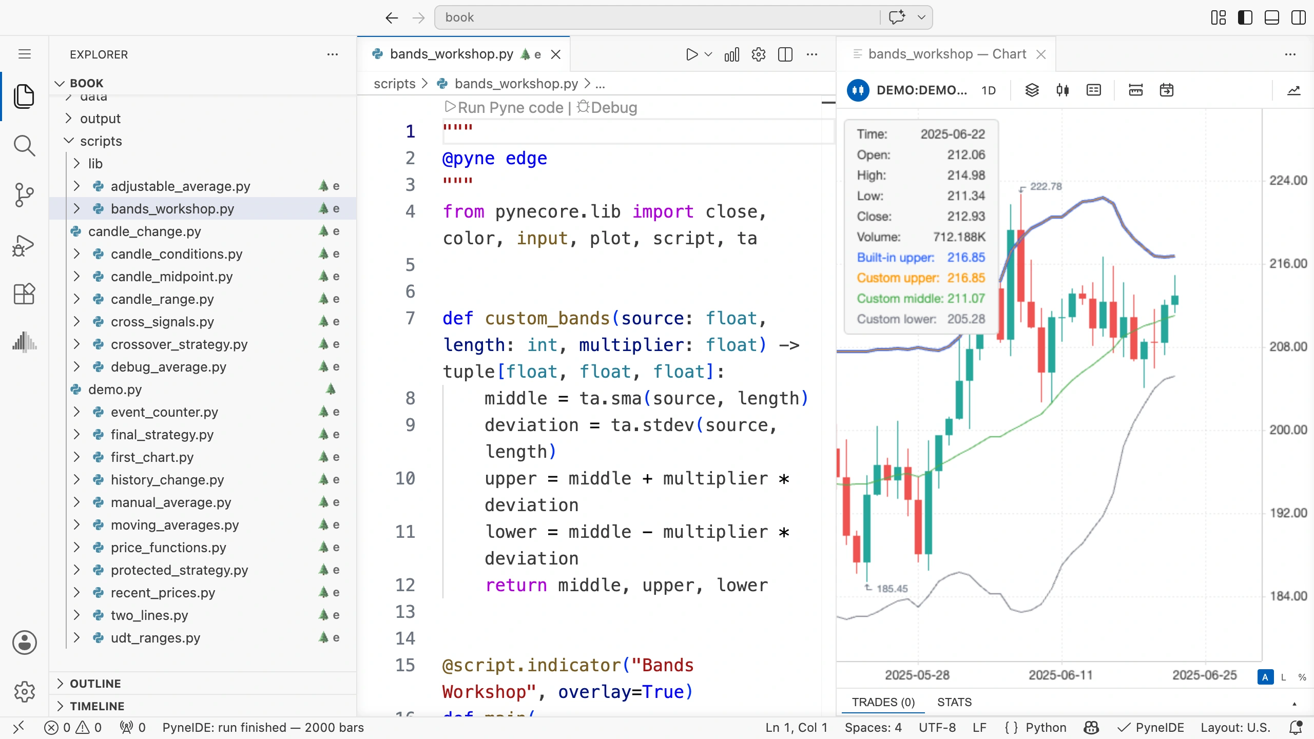
For a more precise check, open the output values with Open plot output CSV on the chart toolbar. For a custom version, check both the first valid point and later values. Lines that look identical can still have small differences.
Try it yourself: an EMA center line
Change only the center line in custom_bands: use an EMA instead of an SMA. Keep the standard deviation calculation and the built-in ta.bb call for comparison.
Before running it, predict: will your upper boundary still overlap the built-in one throughout? What happens after a sudden price change?
Solution
The first calculation line of the custom function:
middle = ta.ema(source, length)We measure both boundaries from this EMA, while the ta.stdev calculation stays the same. Your center line and both boundaries therefore generally shift relative to the original bands. The difference between the two upper values equals the difference between the EMA and SMA, because we add the same standard deviation times the same multiplier to both.
This is now your own experimental variant. A different line alone does not tell you whether a trading rule will perform better with it; you can examine that in a separate strategy with the same data and settings.
Continue exploring the library
Choose an indicator and describe in your own words what data it receives, what it remembers, and what result it returns. Follow its internal calls until you can piece together the calculation. For RSI, for example, following rsi → rma → sma takes you from differences through smoothing to the initial value.
Read the branches for missing values, warmup, and edge cases too. When creating your own version, change one detail first and compare its results with the original. This helps you distinguish an intentional change from a calculation error.
You can access other library functions’ source with the same Command-click or Ctrl-click. A longer indicator may take more time, but the reading approach is the same: inputs, retained data, calculation, result.