Read the backtest results
Check the strategy trade by trade and compare the effect of costs.
Your first strategy has run. Now you examine whether the simulated trades really follow the specified rule and what the displayed results mean.
The book’s demo data is an artificial price series. Its results are useful for checking how a program behaves. They do not establish the expected return on a real market.
Start with one trade
Run crossover_strategy.py with lengths of 5 and 20. Wait for it to finish, then select Trades in the panel below the chart. If the panel is closed, open it with the arrow on its right.
The table lists entry and exit details for each trade. In a long trade, entry is a buy and exit is a sell.
| Column | What does it show? |
|---|---|
Trade | Trade number and entry identifier |
Entry time | Time the entry filled |
Entry price | Price the entry filled at |
Exit time | Time the exit filled |
Exit price | Price the exit filled at |
Qty | Trade quantity |
Profit | Monetary result of the closed trade |
Profit % | Percentage result of the trade |
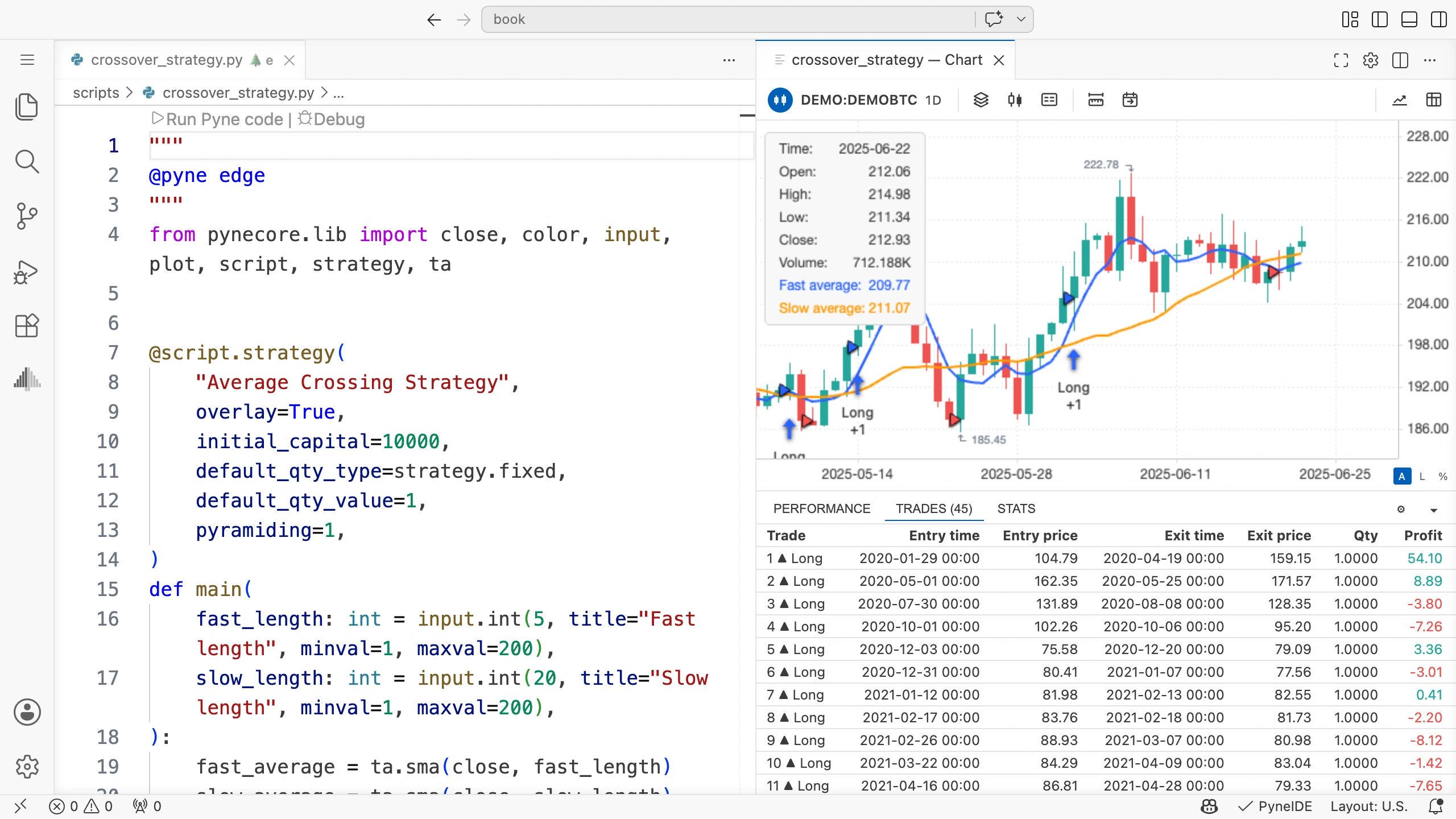
Click a trade row. You can find its period on the chart. Examine both the crossing before entry and the crossing that triggered the close.
The original program did not specify commission_value or slippage, so the baseline run does not include the costs we are about to add separately. First use this simple run to check direction, timing, and quantity.
Calculate the result of a simple trade
If you bought one unit at 100 and sold it at 103, the price difference is 3. With a point value of one and no costs, this is also the monetary result.
More generally, the price-based result of a long trade is:
(exit price − entry price) × quantity × point valuePoint value is part of the market metadata. It describes the monetary value of a one-unit price change for a one-unit position. The book’s DEMO data has a point value of 1.
Commissions reduce the trade’s net result. Slippage changes the fill price, so it is already reflected in the price difference. You do not need to subtract the same slippage again from the adjusted prices.
The Performance view
The Performance tab shows how equity develops over the whole run. The interface includes these fields:
- Cumulative P&L: the change in equity relative to initial capital;
- Max drawdown: the largest decline from an earlier peak of the equity curve being examined;
- Final equity: equity on the run’s last processed candle;
- Max run-up: the largest rise in equity from an earlier low.
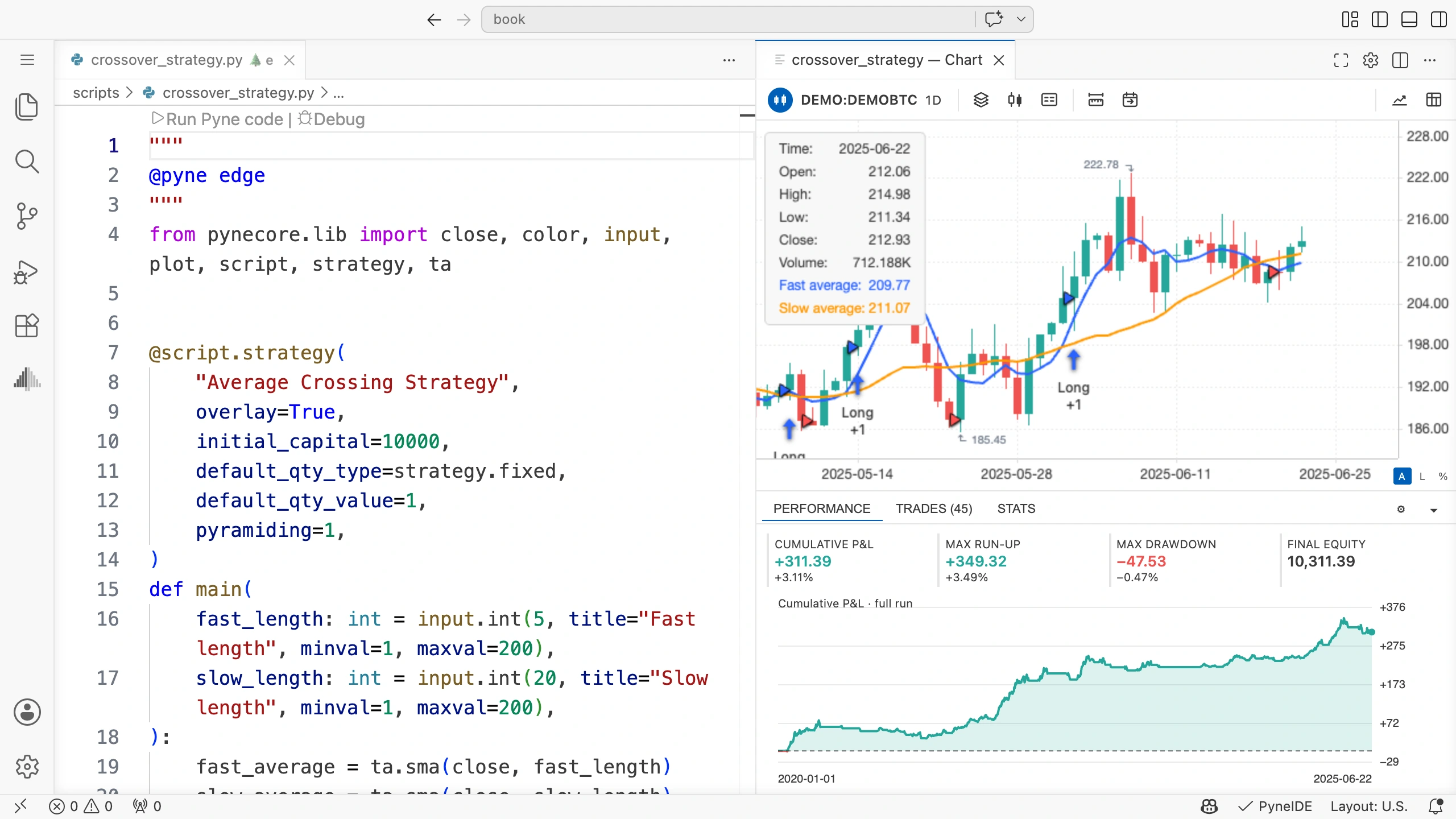
Equity may also include the changing value of an open position. The final equity value therefore does not necessarily equal initial capital plus the sum of closed-trade profits. Check for a position still open at the end of the data too.
Examine the intermediate sections of the equity curve as well as its endpoint. Different drawdowns and long losing periods can lead to the same final result.
The Stats view
The Stats tab shows detailed statistics at the end of the run. Total Trades helps you check the number of closed trades, and Net Profit their combined net result.
Profit Factor is the ratio of the combined results of winning and losing trades: total profit divided by the absolute value of total loss. If there are no losing trades, this ratio is not an ordinary finite number for comparison.
The win rate describes what proportion of closed trades were profitable. It does not determine total profit on its own. A few large losses can outweigh many small wins.
A small number of trades can easily produce a misleading summary. Keep the total trade count alongside the other metrics, and examine individual losing trades too.
Costs in Properties
Use the Strategy properties gear in the chart’s bottom panel to open strategy settings, then select Properties. Here you can change initial capital, quantity, and costs too.
Comparing the next two runs is an exercise. The specified costs are part of the example; costs for a real market must be set separately.
- Check that Initial capital is 10000 and Order size is 1 Contracts.
- Set Commission to 0.1 and choose % of order value as the unit. You can enter it in the field as
0.1. - Set Slippage to 2 ticks.
- Click Save, then start Run Pyne code and wait for it to finish.
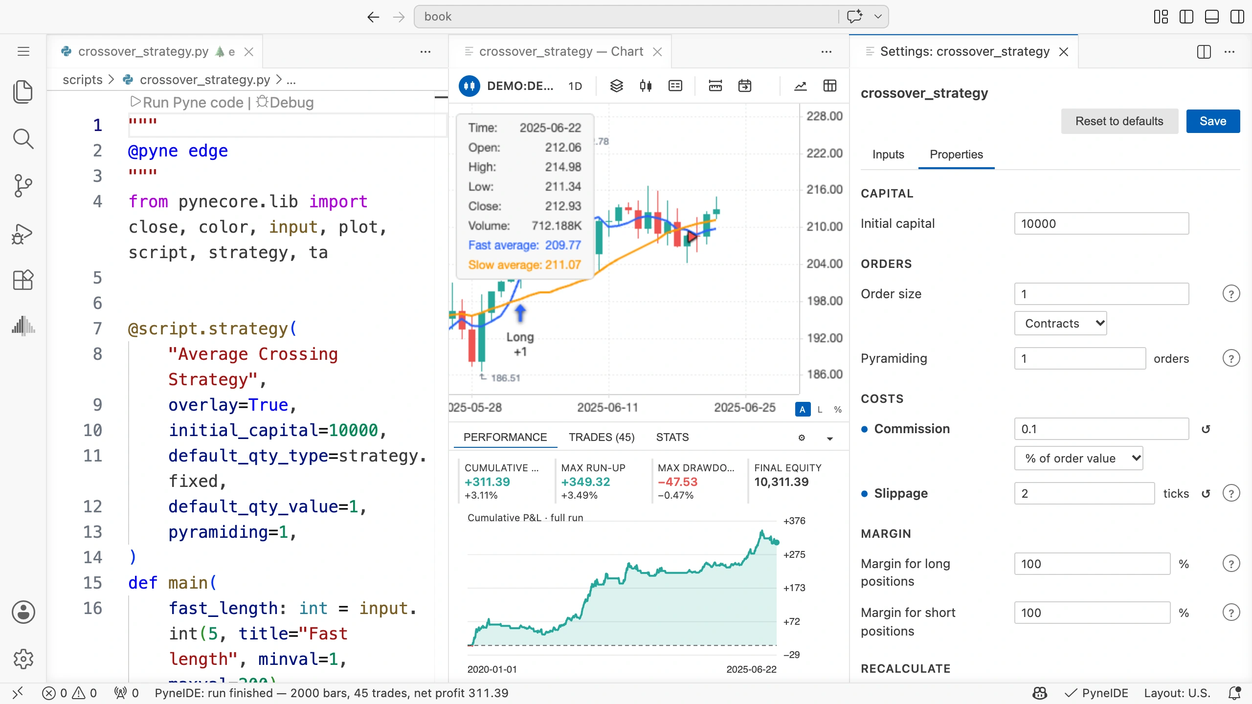
A commission of 0.1 percent is not 10 percent: the field is in percentage units. For a fill worth 100, it means a commission of 0.1. Entry and exit are both fills, and both can incur costs.
A tick is the market’s smallest price increment. In DEMO metadata, it is 0.01, so two ticks mean a price change of 0.02. Slippage moves a market order’s fill price in an unfavorable direction for the strategy.
Other markets can have different tick sizes and point values. Do not automatically carry your interpretation of costs from DEMO data to another instrument.
Fill settings are part of the experiment too
The On bar close setting under Fill orders affects market order timing. For the book’s baseline strategy, leave it off so an order generated by a signal fills at the next open.
After order is filled can request recalculation after a fill. Using bar magnifier can examine intrabar fills with more detailed data from a lower timeframe. These change execution conditions; leave them off when comparing the baseline run.
Changing even one setting produces a new run result. If you change length, quantity, costs, and fill behavior all at once, you cannot tell which caused a difference.
Save what you compared
The chart toolbar’s Open trades output CSV button opens the trade export. Open plot output CSV opens the table of plotted values. You can also find the result files in the project’s Output group.
Before running the same program again, copy any export you want to keep under a different filename. The result filename alone does not identify every setting.
In your own notes, record at least:
| Run | Data | Fast/slow length | Quantity | Commission | Slippage |
|---|---|---|---|---|---|
| Baseline | DEMO | 5 / 20 | 1 unit | 0% | 0 ticks |
| With costs | DEMO | 5 / 20 | 1 unit | 0.1% | 2 ticks |
Add the results you obtain too. Fill in this table in your own notes using actual runs.
Try it yourself
Compare the same trade in the run without costs and the run with costs. Check its entry price, exit price, and profit. What changed, and what stayed the same in the signal rule?
Solution
The moving averages and their crossing are not calculated from commission or slippage, so the underlying signals do not change. Market entry and exit prices can be less favorable due to slippage. Commission further reduces the trade’s net result.
The runs are directly comparable when their inputs, quantity, data, and fill behavior match, and the strategy can execute the orders in both cases.
Select another dataset
After the demo, you can also use PyneIDE’s data downloader to create your own market dataset. The new data may have different prices, tick sizes, quantity limits, and trades. Examine the data first, then compare results.
- In the Pyne view on the left, hover over the Data group header. Click the Download Data… icon that appears, showing a downward arrow from a cloud. This opens the Symbol Browser. You can also access this item by right-clicking the Data header.
- Choose a provider in Provider. The screenshot uses
ccxt; with it, you can choose the specific data source in Broker too. - Enter the market’s name in the filter field. In the screenshot, we select the
BTC/USDspot market fromcoinbase. Check the full symbol: rows with similar prefixes can represent different markets. - Set Timeframe to
1D, and select 365 days back in From. In To, now requests data up to the time of download. - Click Download and wait for it to finish.
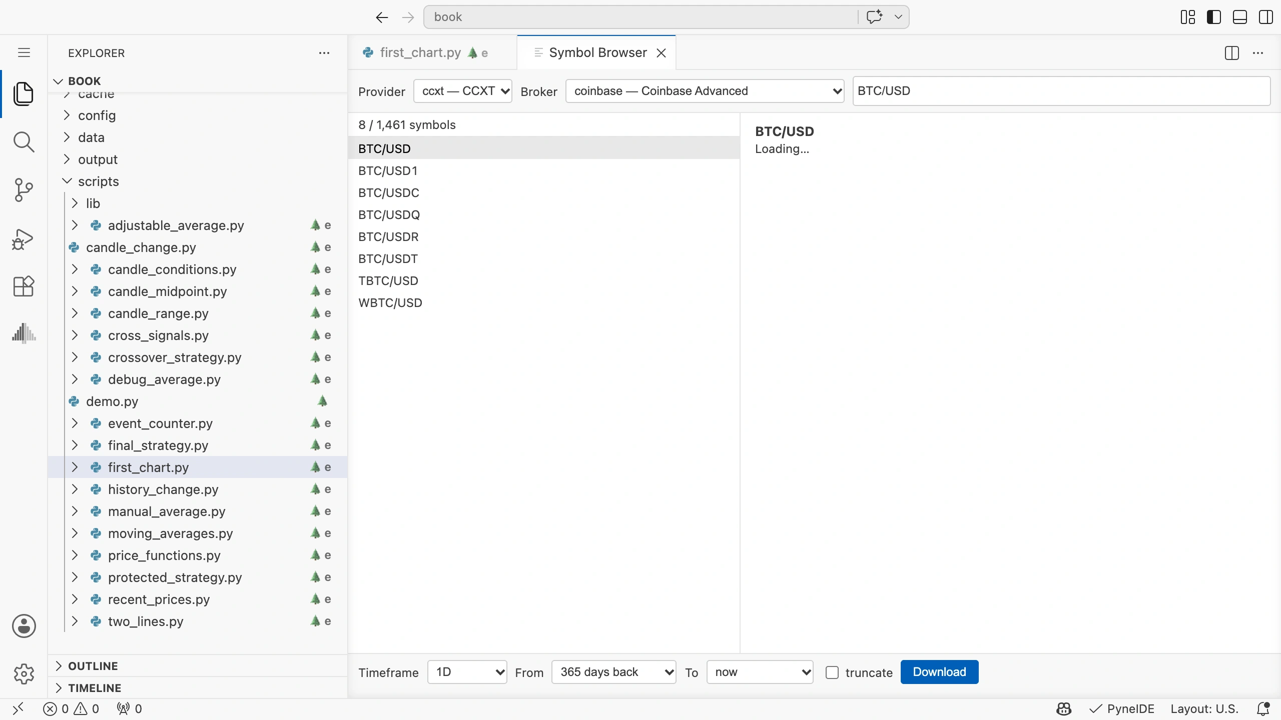
In the information on the right, mintick is the tick size, pointvalue is the point value, and mincontract is the minimum quantity. Check these for your own data too. Data availability and required access depend on the provider; requesting the data selected here does not use a trading account.
The downloaded data goes into the project’s Data group. You can also open the data picker by clicking the market name in the top row of the strategy chart, then select the new data. The chart recalculates; continue to check the inputs and strategy properties.
The download period does not guarantee a particular candle count: the provider’s available history, the market’s trading days, and missing periods all matter. A fresh download can change the dataset being examined, so keep both the data file and its metadata file for comparisons.
Interpret the run
A backtest calculates results from a specified rule, dataset, and execution model together. It helps you check whether the code does what you described and how it would have behaved in that model. Future data is not part of the result.
If you change parameters repeatedly on the same data, you can find a rule fitted to that data. Examining a separate period that you did not use for tuning asks a different question. In the final project, you therefore check program correctness and compare settings separately.